

Random Fatigue Limit: Impetus
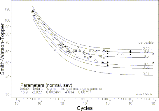
Figure 1: s-N relationship for Ti-6Al-4V illustrating random fatigue limit behavior.
Why a Random Fatigue Limit?
There are at least three practical problems with the traditional, large numbers of s-N tests, approach to estimating fatigue limits:
- At the stress levels of interest, s-N curves are relatively flat. To get failures below the median fatigue limit requires tests that are potentially orders of magnitude longer than the desired cyclic life. The primary interest, of course, is in a stress level at which one percent or fewer of the structures would not survive, say, \(10^7\) cycles. While extrapolation of a median s-N curve to the long life of interest may be acceptable, estimation of the first percentile of the fatigue limit distribution most likely is not.
- The variability of fatigue lives increases greatly as test stresses decrease and a general model for this changing scatter has not been accepted. Thus, extrapolation of the percentiles of the fatigue strength to longer lives also requires correlating the standard deviation of fatigue lives with stress levels.
- Current HCF problems indicate the necessity to define fatigue limits at lives longer than \(10^7\) . The economic burden of testing runout lives to \(10^8\),or longer, only compounds the first two problems.
\( \leftarrow \) Random Fatigue Limit
Because of the enormous scatter in lives at the stress levels of prime interest to HCF, and the expense of testing to very long cycle counts, a better method for estimating and validating fatigue limits is needed.
An innovative approach to describing fatigue limit behavior was proposed recently by Pascual and Meeker. They postulated a random fatigue limit (RFL) model in which each specimen has its own fatigue limit in much the same way that each specimen has its own fatigue lifetime if tested at a sufficiently high stress. This random fatigue limit is explicitly included in the s-N model. Maximum likelihood methods (described elsewhere) are then used to estimate the parameters of the s-N equation as well as the parameters of the fatigue limit distribution. The percentiles of the fatigue limit distribution are easily calculated from the estimated parameters. The random fatigue limit model produces the proper shape of the median s-N function and the type of scatter typically seen in fatigue tests at HCF stress levels, as is illustrated in Figure 1, for Ti-6Al-4V.
Reference: (Pascual and Meeker, “Estimating Fatigue Curves with the Random Fatigue-Limit Model,” TECHNOMETRICS Vol. 41, No. 4, p.277-302, November 1999)