

CLT: fine-print
The CLT is responsible for this remarkable result:
The distribution of an average tends to be Normal, even when the distribution from which the average is computed is decidedly non-Normal. Furthermore, the limiting normal distribution has the same mean as the parent distribution AND variance equal to the variance of the parent divided by the sample size.
Thus, the Central Limit theorem is the foundation for many statistical procedures, including Quality Control Charts, because the distribution of the phenomenon under study does not have to be Normal because its average will be. (see statistical fine print)
Furthermore, this normal distribution will have the same mean as the parent distribution, AND, variance equal to the variance of the parent divided by the sample size.
The Fine-Print:
The distribution of an average will tend to be Normal as the sample size increases, regardless of the distribution from which the average is taken except when the moments of the parent distribution do not exist. All practical distributions in statistical engineering have defined moments, and thus the CLT applies.
Statistical Moments:
Readers have requested further explanation of the fine print, so a slight digression is in order. Statistical Moments are analogous to moments in physics, where we consider a force multiplied by its distance from the centroid or fulcrum. The first statistical moment is the mean, which is the sum of the n distances from zero, times the probability of being at that distance,
\[\mu=\sum_{i=1}^{n}{x_i f(x_i)}\]
If the density is continuous, rather than discrete, the sum becomes an integral,
\[\mu=\int_{-\infty}^{\infty}{x_i f(x_i)} \tag{1} \]
The mean of random variable X is also referred to as the expected value of X, written E X, or E(X).
The variance is the second statistical moment, and is the sum of the squared distances from the mean, times the probability of being at that distance. Higher order moments, skewness (asymmetry) and kurtosis (peakedness) are similarly defined, with the distances, \( (x-\mu) \) raised to the 3\(^{rd}\) and 4\(^{th}\) power, respectively.
Sometimes the Moments Diverge:
The Cauchy is an example of a pathological distribution with nonexistent moments. The density is
\[f(x) = \frac{1}{\pi}\frac{1}{1+x^2},\quad\infty < x < \infty\]
The density looks like this:
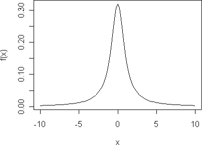
The Cauchy distribution has no statistical moments, like mean and variance.
The Cauchy is a proper density, however, since it integrates to one.
\[\int_{-\infty}^{\infty}{f(x_i)} = 1\]
so that\[F(x) = \int_{-\infty}^{\infty}{ \frac{1}{\pi}\frac{1}{1+x^2} dx}=\frac{1}{\pi}\arctan(x) \bigg|_\infty^\infty=\frac{1}{\pi}\bigg( \frac{\pi}{2}-\frac{-\pi}{2} \bigg)=1\]But the mean (the first statistical moment) doesn’t exist. (In fact, none of the moments exists.) That is, the integral defined by equation (1) diverges. It turns out that showing that the moment integrals do not converge is somewhat complicated. The moment-generating function won’t work since the moment generating function for a Cauchy doesn’t exist. Casella and Berger, however, use a clever computational trick to show that E |X| does not exist and thus neither does E X:$$E|X|= \int_{-\infty}^{\infty}{ \frac{|x|}{\pi}\frac{1}{1+x^2} dx=\frac{2}{\pi}}\int_{0}^{\infty}{\frac{1}{1+x^2} }dx$$Now, for any positive number, M,
$$E|X|= \int_{0}^{M}{ \frac{x}{1+x^2} } dx=\frac{\log(1+x^2)}{2} \bigg|_0^M dx=\frac{\log(1+M^2)}{2} $$
Therefore,
$$E|X|= \lim_{M \rightarrow \infty } \frac{2}{\pi}\int_{0}^{M}{\frac{x}{1+x^2} }dx=\frac{1}{\pi} \lim_{M \rightarrow \infty } \log(1+M^2)=\infty$$
Since E|X| does not exist neither does E X. There mean of the Cauchy density does not exist.
Summary:
The Central Limit Theorem describes the relation of a sample mean to the population mean. If the population mean doesn’t exist, then the CLT doesn’t apply and the characteristics of the sample mean, \(\bar{X}\), are not predictable. Attention to detail is needed here: You can always compute the numerical mean of a finite number of observations from any density (if every observation is finite). But the population mean is defined as an integral, which diverges for the Cauchy, so even though a sample mean is finite, the population mean is not.
The Cauchy has another interesting property – the distribution of the sample average is that same as the distribution of an individual observation, so the scatter never diminishes, regardless of sample size.
Caveat:
The Central Limit Theorem almost always holds, but caution is required in its application. If the population mean doesn’t exist, then the CLT is not applicable. Further, even if the mean does exist, the CLT convergence to a normal density might be slow, requiring hundreds or even thousands of observations, rather than the few dozen in these examples. The prudent practitioner will know the limitations of any rule, algorithm or function, in statistics or in engineering.
Reference:
Casella and Berger, Statistical Inference, 2\(^{nd}\) ed., Duxbury, 2002