R-squared

R-squared

\(R^2\) can be a lousy measure of goodness-of-fit, especially when it is misused. The Akaike Information Criterion (AIC) affords some protection by penalizing attempts at over-fitting a model, but understanding what \(R^2\) is, and what it’s limitations are, will keep you from doing something dumb.

By definition, \(R^2\) is the fraction of the total squared error that is explained by the model. Thus values approaching one are desirable. But some data contain irreducible error, and no amount of modeling can improve on the limiting value of \(R^2\). Sadly, many practitioners, including some who should know better, pursue very high order polynomial models in the mistaken but widely held belief that as the number of parameters approaches the number of observations, the model can be made to pass through every point. (It appears that the origin of this misconception is, as with many difficulties with applied statistics, not reading the fine print.)

Here is an example. The data are real. Repeated testing under nominally identical conditions results in considerable variability in measured material strength. These specimen-to-specimen differences are real and result from uncontrollable, and sometimes immeasurable, deviations in material characteristics such as chemistry, microstructure, processing, or fabrication. (It is a common oversight to suppose that all of the variables you can measure includes all that have an influence.)

Thus, it is fruitless trying to “explain” this random variability in material response using increasingly involved functions of test temperature, since temperature can only account for the central behavior, and not deviations from it.

\(R^2\) is a Lousy Criterion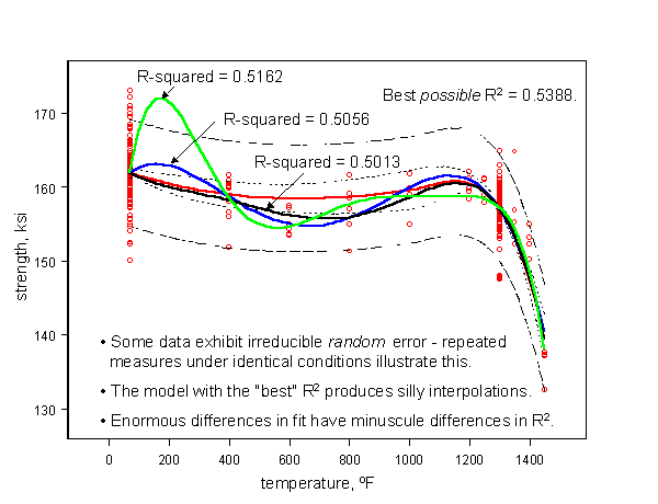

One alarming consequence of choosing the “best” model because it has an incrementally higher \(R^2\), is how poorly it can be expected to behave when used to predict behavior at conditions for which there are no data, like 150F in this example.

While the lesson seems obvious in this example, the problem can appear in any collection of observations containing a large random component. Thus, one of the early steps in model building should be to determine how much of the observed variability is irreducibly random*.

* Furthermore, in some situations the random error may exhibit autocorrelation in time and/or space. This necessitates more sophisticated modeling since most common statistical regression packages require the errors to be uncorrelated (and normal).