CLT: Triangular Distribution
The CLT is responsible for this remarkable result:
The distribution of an average tends to be Normal, even when the distribution from which the average is computed is decidedly non-Normal. Furthermore, the limiting normal distribution has the same mean as the parent distribution AND variance equal to the variance of the parent divided by the sample size.
Thus, the Central Limit theorem is the foundation for many statistical procedures, including Quality Control Charts, because the distribution of the phenomenon under study does not have to be Normal because its average will be. (see statistical fine print)
Example: Triangular Distribution
 | The triangular distribution on the left is obviously non-Normal. Call that the parent distribution. |
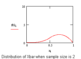 | To compute an average, Xbar, two samples are drawn, at random, from the parent distribution and averaged. Then another sample of two is drawn and another value of Xbar computed. This process is repeated, over and over, and averages of two are computed. The distribution of averages of two is shown on the left. |
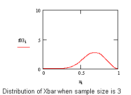 | Repeatedly taking three from the parent distribution, and computing the averages, produces the probability density on the left. |
 | Repeatedly taking four from the parent distribution, and computing the averages, produces the probability density on the left. |
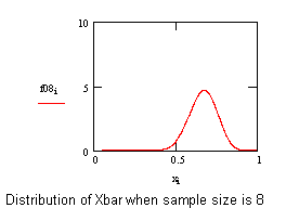 | Repeatedly taking eight from the parent distribution, and computing the averages, produces the probability density on the left. |
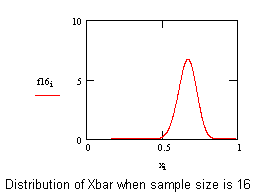 | Repeatedly taking sixteen from the parent distribution, and computing the averages, produces the probability density on the left. |
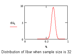 | Repeatedly taking thirty-two from the parent distribution, and computing the averages, produces the probability density on the left. |
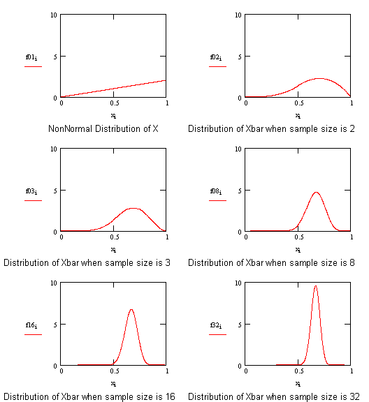 | Notice that when the sample size approaches a couple dozen, the distribution of the average is very nearly Normal, even though the parent distribution looks anything but Normal. |
Statistical fine-print:
The distribution of an average will tend to be Normal as the sample size increases, regardless of the distribution from which the average is taken except when the moments of the parent distribution do not exist. All practical distributions in statistical engineering have defined moments, and thus the CLT applies.
The Cauchy is an example of a pathological distribution with nonexistent moments. Thus the mean (the first statistical moment) doesn’t exist. If the mean doesn’t exist, then we might expect some difficulties with an estimate of the mean like Xbar.
(Click here for even more fine print.)
