“In theory there is no difference between Theory and Practice.
In practice, there is.”

 

How FORM/SORM is Supposed to Work

part 2 of 4

 

FORM (First Order Reliability Method) has been used extensively by engineers for nearly two decades. What has been studiously ignored, however, is how well FORM/SORM assumptions hold up in describing real data.

It is standard practice to illustrate the idea with only a one-dimensional demand and a one-dimensional capacity so that the concept can be plotted in a n=2 dimensional plot, like Figure 1

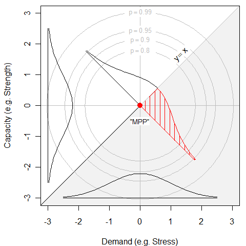
Figure 1  90%, 90%, 95% and 99% concentric circles of the bivariate normal density. The MPP appears as a red dot.

 
The g-function as the line where capacity=demand exactly, an admittedly poor design having a 50% failure rate.

The density is centered at (0, 0). The bivariate density is bisected again by the b g-function. A standard normal density is plotted along that line, and the probability of the “most probable point” is indicated by the shaded region in the lower right. Anything below the y=x line (i.e. Capacity < Demand) will fail.
While it may appear that the bivariate normal density is formed by rotating a univariate normal density, that is not the case. The density of the one-dimensional standard normal distribution at x=0 is oneOvrSqrt2pi.gif. The density of the two-dimensional standard normal distribution at (x=0, y=0) is oneOvr2pi.gif, as it must be so that its double integral equals one. For an n-dimensional standard multivariate normal density the maximum ordinate at the origin is oneOvrKroot2pi.gif. In summary: the MVN is not simply a rotation of the standard Normal. The foundation of NESSUS is built on sand.

Of course a design having capacity exactly equal to its demands would have an unacceptably high failure rate of 50%. To remedy this we must either increase the capacity or decrease the demand, in either case thus redefining the joint probability density such that the new g-function is now a line where demand=capacity-. can be selected to provide the desired failure rate. Since we are comparing the first 7 of 68 real laboratory specimen failures, we choose to make Pfail=10%. This has the effect of moving the joint probability density to a new mean = (0, ). It is convenient (but confusing) to re-define the origin to be (0, 0) as before, which means that the g-function is no longer shown as a line partitioning failures from non-failures and where demand equals capacity, going through (0, 0), but rather going through (0, ) and having the desired failure rate (10% here). In other words we have redefined failure to be “having as margin less than ” rather than “fails.”