Random Fatigue Limit
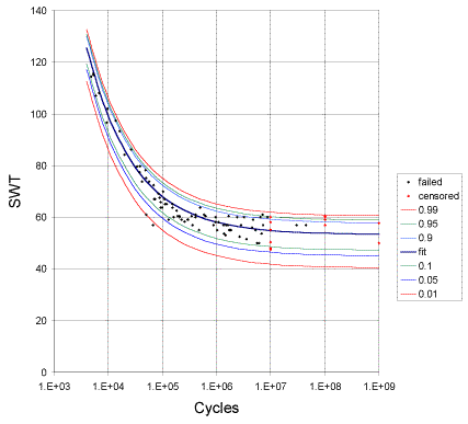
 Figure 1: s-N relationship for Ti-6Al-4V illustrating random fatigue limit behavior.
In the LCF region (upper left, \(N<10^7\) cycles) it has long been sound engineering practice to read the curve at some operating level (stress, strain, SWT, or similar metric) and count cycles until the lower bound cycle count was exceed and the component would be retired from further service. With the recognition of the random fatigue limit comes the necessary, but unpopular, realization that similar cycle counting in the HCF region of the s-N curve (lower right, \(N \gg 10^7\) cycles) isn’t feasible because the behavior of a given specimen, or component, depends on its own unique fatigue limit. For example, reading the curve at SWT=50 shows the behavior of some specimens with lower individual fatigue limits to have failed, while others, tested at the same stress level, ran out, producing censored observations, where actual failure time is unknown other than being greater than the censoring cycle count. Counting the cycles exhausted at SWT=50, then, would depend on knowing the individual RFL, which of course, being random, is unknowable a priori. Thus what is sound engineering practice in the LCF region is not feasible for HCF. This is only a modest setback, however because the RFL model proves a method of estimating the probability of failure, even if the cycle count is intractable.
The RFL Model is a Precursor to a “Probabilistic Goodman” Diagram.
The next step is to consolidate the s-N behavior described by the RFL model and illustrated in Figure 1, into a “Probabilistic Goodman”(1) diagram. It should be recognized that while this step will be a welcome advance, it will not be the ultimate destination. There is much more to the behavior of a material responding to HCF than can be described using only the mean stress, alternating stress measure of the Goodman approach.
Summary:
HCF data are characterized by more than just runouts (described elsewhere). Tests of \(10^7, 10^8\) and
even \(10^9\) cycles often display an asymptotic behavior, illustrated in figure 1.
Heretofore analyzing these data produced unsatisfactory results as the usual assumption of uniform variance (data scatter), over the many orders of magnitude in fatigue life, proved untenable. Attempts to deal with this ballooning variance by various variance-stabilizing transformations were similarly unsuccessful, as were attempts to model the behavior with a single-valued fatigue limit asymptote.
The difficulty is that the fatigue limit exhibited in a given s-N test is not a constant, as had been previously thought, but rather a random variable, just as the individual fatigue life of a specimen tested at a given stress is random. While this may seem self-evident in retrospect, it was only very recently recognized and described mathematically.
Alas, the devil IS in the details. While understanding the idea of a random fatigue limit is simple enough, estimating the parameters of such a model is a challenging task indeed.
Professor William Q. Meeker has graciously made his RSplida software, including the R codes used in his excellent book (below), available to all. To get the software visit his website:
http://www.public.iastate.edu/~wqmeeker/
Footnote:
\(^{(1)}\) Goodman diagrams have been called Goodman diagrams for over a hundred years since Goodman popularized the idea of plotting constant life lines as a function of alternating and mean stresses. Recently revisionists have taken to referring to these curves as Haigh diagrams because Goodman was not the first to use such curves; this now being attributed to Haigh. This presents an interesting example of Stigler’s Law of Eponymy, which states that: “No scientific discovery is named after its original discoverer.” Stigler notes that he, himself, didn’t discover this phenomenon, and thus feels quite justified in applying his name to it.
References:
- Pascual and Meeker, “Estimating Fatigue Curves with the Random Fatigue-Limit Model,” TECHNOMETRICS Vol. 41, No. 4, p.277-302, November 1999
- Stephen M. Stigler, Statistics on the Table, a history of statistical concepts and methods, Harvard University Press, Cambridge, MA, 1999, p277-290.
- Meeker and Escobar, Statistical Methods for Reliability Data, Wiley, 1998. This is a wonderful book. If your bookseller is out of stock, you can get it quickly from amazon.com.

