Joint, Marginal, and Conditional Distributions
We engineers often ignore the distinctions between joint, marginal, and conditional probabilities – to our detriment.

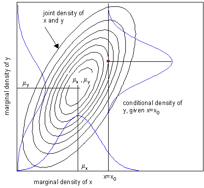
Figure 1 – How the Joint, Marginal, and Conditional distributions are related.
Joint probability is the probability of two or more things happening together. \(f(x, y \mid \theta)\) where \(f\) is the probability of \(x \text{ and } y\) together as a pair, given the distribution parameters, vector theta. Often these events are not independent, and sadly this is often ignored. Furthermore, the correlation coefficient itself does NOT adequately describe these interrelationships.
Consider first the idea of a probability density or distribution: \(f(x \mid \theta)\) where \(f\) is the probability density of \(x\), given the distribution parameters, \(\theta\). For a normal distribution, \(\theta=(\mu, \sigma)^T\) where \(mu\) is the mean, and \(sigma\) is the standard deviation. This is sometimes called a pdf, probability density function. The integral of a pdf, the area under the curve (corresponding to the probability) between specified values of \(x\), is a cdf, cumulative distribution function, \(F(x, \mid \theta)\). For discrete \(f , F\) is the corresponding summation.
A joint probability density two or more variables is called a multivariate distribution. It is often summarized by a vector of parameters, which may or may not be sufficient to characterize the distribution completely. Example, the normal is summarized (sufficiently) by a mean vector and covariance matrix.
marginal probability: \(f(x, \mid \theta)\) where \(f\) is the probability density of \(x\), for all possible values of \(y\), given the distribution parameters, vector \(\theta\). The marginal probability is determined from the joint distribution of \(x \text{ and } y\) by integrating over all values of \(y\), thereby “integrating out” the variable \(y\). In applications of Bayes’s Theorem, \(y\) is often a matrix of possible parameter values. Figure 1 illustrates joint, marginal, and conditional probability relationships.
conditional probability: \(f(x \mid y, \theta)\) and theta where where \(f\) is the probability of \(x\) by itself, given specific value of variable \(y\), and the distribution parameters, \(\theta\). (See Figure 1) If \(x \text{ and } y\) represent events \(A\) and \(B\), then \(P(A|B) = n_{AB}/n_{B}\) , where \(n_{AB}\) is the number of times both \(A\) and \(B\) occur, and \(n_B\) is the number of times \(B\) occurs. \(P(A|B) = P(AB)/P(B)\), since \(P(AB) = n_{AB}/N\) and \(P(B) = n_B/N\) so that
\[PA|B = \frac{n_{AB}/N}{n_B/N} = n_{AB}/n_B\]
Note that in general the conditional probability of \(A\) given \(B\) is not the same as \(B\) given \(A\). The probability of both \(A\) and \(B\) together is \(P(AB)\), and if both \(P(A)\) and \(P(B)\) are non-zero this leads to a statement of Bayes Theorem:
\[P(A \mid B) = P(B \mid A) \times P(A) / P(B)\] and \[P(B \mid A) = P(A \mid B) \times P(B) / P(A)\]
Conditional probability is also the basis for statistical dependence and statistical independence.
Independence: Two variables, \(A\) and \(B\), are independent if their conditional probability is equal to their unconditional probability. In other words, \(A\) and \(B\) are independent if, and only if, \(P(A \mid |B)=P(A)\), and \(P(B \mid A)=P(B)\). In engineering terms, \(A\) and \(B\) are independent if knowing something about one tells nothing about the other. This is the origin of the familiar, but often misused, formula \(P(AB) = P(A) \times P(B)\), which is true only when \(A\) and \(B\) are independent.
conditional independence: \(A\) and \(B\) are conditionally independent, given \(C\), if
\[Prob(A=a, B=b \mid C=c) = Prob(A=a \mid C=c) \times Prob(B=b \mid C=c)\] whenever \(Prob(C=c) > 0\).
So the joint probability of \(A B C\), when \(A\) and \(B\) are conditionally independent, given \(C\), is then
\(Prob(C) \times Prob(A \mid C) x Prob(B \mid C)\). A directed graph illustrating this conditional independence is \(A \leftarrow C \rightarrow B\).

