There are more complicated definitions, like …

“The density function of continuous random variables, \( \textbf{X}=X_1, X_2, X_3, \dots ,X_n \) that depend on model parameters, \(\theta = \theta_1, \theta_2, \theta_3 \dots, \theta_k \), and written as \(f(\textbf{X}|\bf{\theta})\), is the probability density function of \(\textbf{X}\), given \(\theta\), or as the likelihood of \(\mathbf{\theta}\) given \(\textbf{X}\), often written as \( \textbf{L}(\theta | \textbf{X}\))”

(Which definition do you prefer? Me too.)

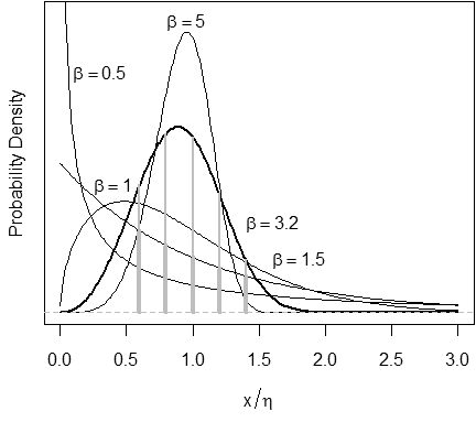
Figure 1 – Some values of Weibull \(\beta\) are more likely than others.

 

Probability

We engineers recognize the figure above as a familiar “probability density function,” and see it as a function of the random variable, \(x\) . For a given \(x\), the ordinate, \(y\), is the probability that \(x\) can take on that value.

Well, that’s not quite right. As it turns out the probability that \(x\) can take on EXACTLY some value \(x_0\) is precisely zero! For example, if \(x_0\) is exactly 1, then the value of \(x=1.00000000000000001\) is excluded. You can see that a vanishingly small difference is still a difference and so the probability of exactly some value must be zero.

Wait! Don’t panic! The probability that \(x\) is within some non-zero distance of \(x_0\) is the ordinate, \(y\), times the interval of \(x\) that we say is close enough, \(\delta x\). So the probability of \(x\) being within that interval is the integral of the probability curve from \(x-\Delta x/2\) to \(x+ \Delta x/2\) (You can also see that if \(\Delta x\) is zero then the product of zero and the ordinate, \(y\), is zero too.)

So what?

There is another way to interpret the figure. Rather than consider \(x\) as unknown and \(y\) as the probability that \(x\) is within some interval, we could also consider \(x\) as known, and \(y\) as the probability (or “likelihood”) that we put the curve in the right place, i.e., that we have the right value for Weibull \(\eta\), the distribution’s location parameter, and that we have the right shape parameter,Weibull \(\beta\), too.

Likelihood

The figure here compares the likelihood values for \(\beta=1.5\) (wide vertical lines) and \(\beta=3.2\) (narrow lines) at \(x=0.6, 0.8, 1.0, 1.2, \text{ and } 1.4\). In this example, a value of 3.2 for the Weibull shape parameter, \(\beta\), is more likely than a value of 1.5, given the known values of \(x\).

We would multiply the likelihoods for each x observation to compute an overall likelihood for Weibull beta. Since multiplication of likelihoods can be messy, in practice we sum the logs of the likelihoods. (The maximum loglikelihood will occur at the same value for Weibull beta as the maximum for the likelihood itself because the logarithm is a monotonic function.)

This is the maximum likelihood criterion. It says that we should choose values for the Weibull model parameters, \(\eta\) and \(\beta\), that maximize the likelihood (probability) that the experiment turned out the way that it did. Although maximum likelihood estimators (MLEs) are sometimes biased, they often more than make up for that by having smaller variability, and thus are superior to other methods for estimating model parameters. (More on that topic here.)

---

The statistical literature often uses “likelihood” and “loglikelihood” interchangeably, which can be confusing to the statistical newcomer, but in practice it is rather easy to distinguish the two based on context.