Round-Robin Testing

Round Robin testing can sometimes make you see something that isn’t there.

Here is an example of purely random behavior that certainly appears to be anything but random.

We will draw 60 random samples from the same lognormal distribution\(^1\) of “cycles-to-failure.” We will label the first 3 samples “laboratory 1,” the next 3 samples “laboratory 2,” and so on up to “laboratory 20.”

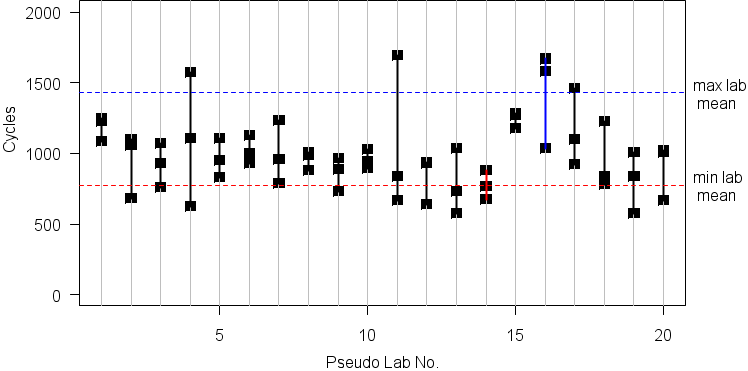
Next we plot the “results” for each of the 20 “laboratories.”

From the plot we can draw these conclusions:

• The “best” lab’s results have a mean twice the “worst” lab’s results.
• Two labs (4 and 11) have “abnormally” large scatter, caused by poor quality control.
• Labs 1, 8, 10, and 15 have “superior” quality control resulting in very little testing scatter.

ALL OF THESE CONCLUSIONS ARE BOGUS! … because these are just 60 random numbers from the same distribution, randomly grouped in threes.

Let’s take a closer look.

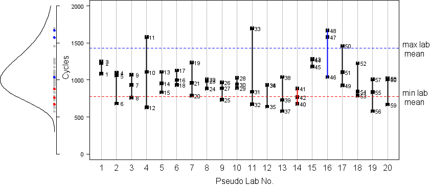
The following figure shows the sequence in which the 60 random number were sampled, and plots all of them along with their parent density, on the left. It is obvious that these are simply 60 random numbers, and grouping by laboratory (1,2,3, 4,5,6, … 58,59,60) is completely arbitrary and has no statistical significance.

So what?

Engineers often “test for statistical significance” using an \(\alpha = 0.05\) criterion. But 5% is 1 out of 20, and if we have 20 random samples then we might expect to find a “significant” happening that is, in reality, only happenstance. In real-world round robin testing it is vital to distinguish between real lab-to-lab differences and apparent differences arising from chance.

Statistical Analysis:

For this simple example we know the result in advance because this is only a numerical simulation. We don’t need a statistical model to test for lab-to-lab significance because we know that there isn’t any – even though it may look like there is. But what about real situations where we only have the laboratories’ round robin results? What then?  (Perhaps you may wish to give me a call? Even better: Call me before you spend a lot of money collecting data that may not be able to distinguish the differences you’re looking for.)

Notes:

\(^1\)   The parent density is lognormal with mean \( \bar X = \log_{10}(1000) \; \text{cycles} = 3\),
      with standard deviation \(\hat{\sigma} = 0.13 \; \log_{10} \text{cycles}\).