Wrong Grid (part 2)
Choosing the wrong grid can undermine your analysis, mislead your audience, and make you look foolish.
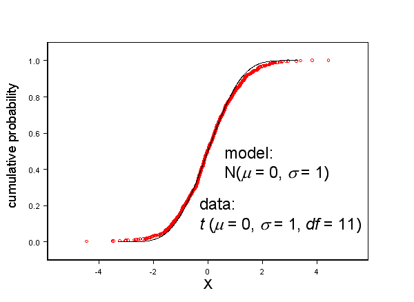
I claim that my statistical model fits the data remarkably well, as shown in Figure 1.
The model agrees with the data very well near the center, deviates very slightly away from the center, but describes the distribution “tails” remarkably well.
This model has to be considered nearly optimal for describing these data.

Figure 1, Statistical model describes the data very well.
Or does it?
To those familiar with statistics, the Cartesian cumulative probability axis is a very poor choice because it obscures the most important behavior, that of the distribution’s “tails.”
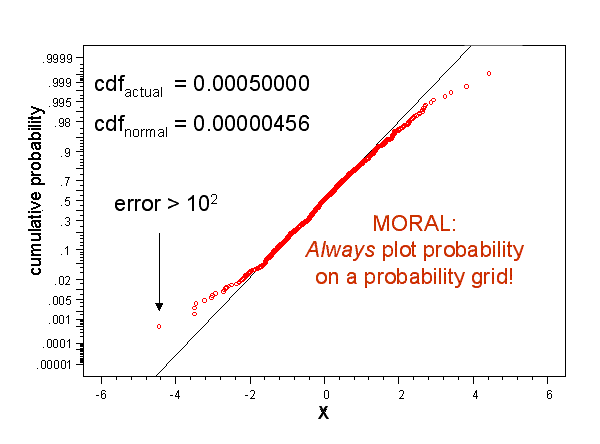
Anyone truly knowledgeable would ask to see the model presented on a more appropriate axis because probability is ALWAYS shown on some form of probability grid, and never * on a Cartesian axis. Figure 2 presents the same data, and the on more appropriate axes.

Figure 2 ,Model performance can be obscured by choice of grid.
My statistical model is inadequate in the tails (where I claimed it performed best), exhibiting errors in excess of two orders of magnitude. Just as a Cartesian grid obscures what is obvious on a logarithmic grid, it also obscures what is obvious on a probability grid. (For an easy way to make your own probability grid, click here.)
Employing a Cartesian grid inappropriately could lead those familiar with the topic to believe that you are either ignorant, for not knowing any better when you should have, or a charlatan for trying to hide deficiencies in your analysis.
Surprisingly, there are some who say, “\(10^{-4}, \, 10^{-6}\) ? Who cares?” For practical purposes they’re both zero.
If these numbers represented your product’s failure rate, then the first case’s warranty costs would be one hundred times those of the second case’s costs. Who cares? You should.
____________________
* As with all rules there are exceptions. If you don’t know what they are then follow the rule.
What has this to do with Engineering?

