There is a continuing debate among statisticians, little known to those outside the field, over the proper definition of probability. The frequentist definition sees probability as the long-run expected frequency of occurrence. \(P(A) = n/N\), where \(n\) is the number of times event \(A\) occurs in \(N\) opportunities. The Bayesian view of probability is related to degree of belief. It is a measure of the plausibility of an event given incomplete knowledge. As can be imagined, if the two schools can’t agree on this, there may be some friction elsewhere as well. Participating in this deliberation is counterproductive. Much of the acrimony between the two schools is over how to describe a prior distribution to represent ignorance. Since there is no disagreement on the veracity of Bayes’s Theorem, I suggest the pragmatic approach: If we have, or can get, an appropriate, informative Bayesian prior, we will use it.
Bayesian philosophy is based on the idea that more may be known about a physical situation than is contained in the data from a single experiment. Bayesian methods can be used to combine results from different experiments, for example. In other situations, there may be sound reasons, based on physics, to restrict the allowable values that can be assigned to a parameter. For example material strength must be nonnegative. Bayesian techniques can help here as well. But often the data are scarce or noisy or biased, or all of these. Experimental results are compared with predicted values, and observing a difference, the predictions are “corrected” by arbitrarily subtracting off the discrepancy. When new data are collected, these too disagree with predictions, and another “correction” is applied, leading to an aggregate of ad hoc tweaks, certainly not Best Practice, however common. Bayesian methods can be used here too, avoiding these spurious heuristics.

How Bayes’s Theorem Works:

Bayes’s Theorem begins with a statement of knowledge prior to performing the experiment. Usually this prior is in the form of a probability density. It can be based on physics, on the results of other experiments, on expert opinion, or any other source of relevant information. Now, it is desirable to improve this state of knowledge, and an experiment is designed and executed to do this. Bayes’s Theorem is the mechanism used to update the state of knowledge to provide a posterior distribution. The mechanics of Bayes’s Theorem can sometimes be overwhelming, but the underlying idea is very straightforward: Both the prior (often a prediction) and the experimental results have a joint distribution, since they are both different views of reality.

Let the experiment be \(A\) and the prediction be \(B\). Both have occurred, \(AB\). The probability of both \(A\) and \(B)\) together is \(P(AB)\). The law of conditional probability says that this probability can be found as the product of the conditional probability of one, given the other, times the probability of the other. That is

\(P(A|B) \times P(B) = P(AB) = P(B|A) \times P(A)\)

if both \(P(A)\) and \(P(B)\) are non zero.

Simple algebra shows that:
\[P(B|A) = P(A|B) \times P(B) / P(A) \tag{1}\]

This is Bayes’s Theorem.

In words this says that the posterior probability of \(B\) (the updated prediction) is the product of the conditional probability of the experiment, given the influence of the parameters being investigated, times the prior probability of those parameters. (Division by the total probability of \(A\) assures that the resulting quotient falls on the \([0, 1]\) interval, as all probabilities must.)

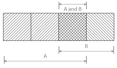
The following example Venn diagram can help keep all this straight.

\(P(A) = 3/4 \text{ (unconditional)}\)

\(P(B) = 2/4 \text{ (unconditional)}\)

\(P(A \text{ and } B) = P(AB) = 1/4 \text{ (joint)}\)

\(P(A \mid B) = P(AB) / P(B) = (1/4)/(2/4) = 1/2\)
\(\quad \text{(conditional probability)}\)

\(P(B \mid A) = P(AB)/P(A) = (1/4)/(3/4) = 1/3 \)

Figure 1: Venn Diagram illustrating Unconditional, Conditional, and Joint Probabilities. (Note that the conditional probability of A, given B is not, in general, equal to the conditional probability of B, given A.)

Bayes’s Theorem for a single continuous random variable

The mathematics in equation 1 assumes that events \(A\) and \(B\) each have a single probability. While true in many cases, in most situations the events are better described with probability densities. The underlying idea is still the same, but the arithmetic can become tedious rapidly. Until recently (the past few decades) computational difficulties were a severe impediment to the utility of Bayes’s methods. Current ubiquitous inexpensive computing power has greatly mitigated this difficulty.

Let \(P(\theta)\) be the prior distribution of some parameter, \(\theta\). It is what is known about \(\theta\) before the data, \(x\), are collected. \(P(\theta \mid x)\) is the posterior distribution of theta, and is what is known later, given the knowledge of the data. Bayes’s Theorem for a single continuous random variable is then:

\[P(\theta \mid x)=\frac{P(x \mid \theta P(\theta)}{P(x)} \quad \tag{2}\]

where the denominator is

\[P(x) = \int{P(x \mid \theta)P(\theta) d\theta}\]

The idea can be expanded for any number of variables, but the resulting integration is often tedious.