That means some statistical model parameters are more likely than others because they explain the observed failures better than other values. We choose the “best” parameter values, i.e. those that maximize the likelihood, which are called, not surprisingly, “maximum likelihood parameter estimates.”  We’ll use the Weibull as an example.

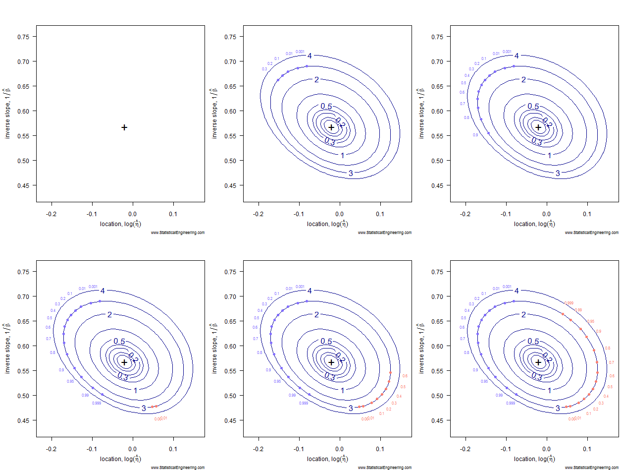
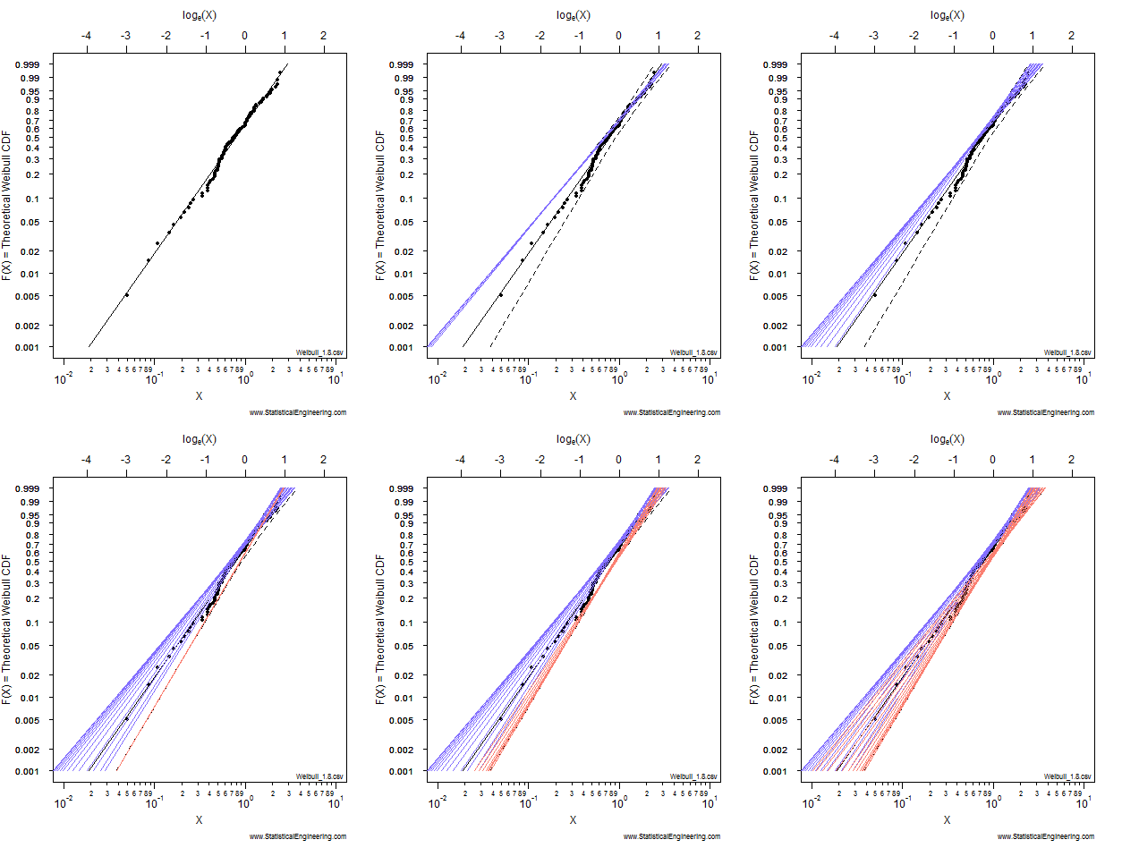
The most likely parameter values, given the data, for the Weibull slope, \(\beta\), and location, \(\eta\), are the “+” in Figure 1, but other values are also plausible, although less likely. That (\(\beta, \eta\)) pair produces the best fit of the data, shown as the black line in Figure 2.

The example below is for a complete dataset, with no censoring. Notice that (after transformation) the confidence “ellipse” is nearly elliptical. Notice, too, that it is not a true ellipse because it is not symmetric along its major and minor axes. That is why we choose not to use methods that employ an ellipse to approximate the loglikeihood surface (like inverting the Fisher Information Matrix) and use the true loglikelihood instead.

Each point along the 95% confidence contour of the loglikelihood surface (Figure 1) produces a Weibull line (Figure 2).

The animated figures illustrate how the model parameters (left figure) control the behavior of the Weibull model (right figure). The “\(+\)” plots the maximum likelihood estimates for (Weibull \(\eta\), Weibull \(\beta\) ), and is represented by the black Weibull line. But values near the “\(+\)” are not unreasonable and we can use the chi-square \(\chi^2\) criterion to gauge “reasonableness.” (More on this later.)

The pseudo-ellipse on the left translates to the confidence bounds on the right, which are constructed one (Weibull \(\eta\), Weibull \(\beta\) ) pair at a time. For each point on the left there is a corresponding line on the right.

Watch to see how the critical isocline on the loglikelihood surface is traversed. Each point represents a \(F(X)\) probability on the right where the Weibull fit is as far away from the MLEs as possible while still remaining “reasonable.” The locus of all such “not unreasonable” lines forms the loglikelihood ratio confidence bounds on the Weibull model.

Because the log of the ratio of likelihoods tends toward a chi-square distribution asymptotically (i.e. as the sample size increases), we have a criterion, chi-square, for constructing confidence bounds on the Weibull model.