The average of \(n\) samples taken from any distribution with finite mean and variance will have a normal distribution for large \(n\). This is the CLT.

The largest member of a sample of size \(n\) has a LEV, Type I largest extreme value distribution, also called Gumbel distribution, regardless of the parent population, IF the parent has an unbounded tail that decreases at least as fast as an exponential function, and has finite moments (as does the normal, for example).

The LEV, has pdf given by

\[f(x \lvert \theta_1, \theta_2) =\frac{1}{\theta_2} \exp\big(-z – \exp(-z) \big)\]

where \(z = (x-\theta_1)/\theta_2 \text{ and } \theta_1, \theta_2\) are location and scale* parameters, respectively and \(\theta_2 \gt 0\).

Similar sampling of the smallest member of a sample of size \(n\) produces an SEV, Type I smallest extreme value distribution, with density

\[f(x \lvert \theta_1, \theta_2) =\frac{1}{\theta_2} \exp\big(z-\exp(z) \big)\]

as \(n\) increases.

There are two other extreme value distributions. If not all moments exist for the initial distribution, the largest observation follows a Type II or Frechet distribution. If the parent density has a bounded tail, the smallest observation in a sample of size \(n\), has a Type III, or Weibull distribution of minima, as \(n\) increases. Examples are smallest samples taken from lognormal, Gamma, Beta or Weibull distributions.

The Weibull distribution is most easily described by its cdf:

\[F(x\vert \eta, \beta) = 1-\exp\Big(-(x/\eta)^{\beta}\Big)\]

where \(\eta\) is the scale (not location) parameter, and \(\beta\) is the shape parameter. Weibull is not a location, scale density*.

Notice that if \(x\) has a Weibull distribution, then \(\log_e(x) \) is SEV, so SEV is to Weibull, as normal is to lognormal.  In other words, SEV is log(Weibull).

Type I and Type III limiting distributions are useful in describing physical phenomena where the outcome is determined by the behavior of the best, or worst, in the sample.

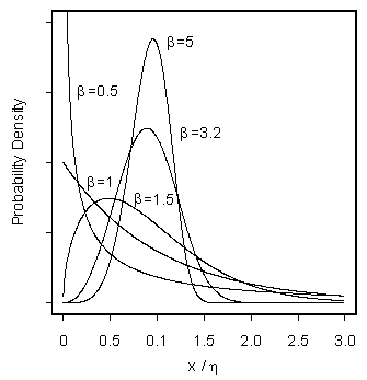
The Weibull Distribution Has Considerable Flexibility.

 

Notes:

* A probability density is a location, scale density if it can take the form of

\(Prob (X \le x) = F(x \lvert \theta_1, \theta_2) = \Phi\big((x-\theta_1)/\theta_2\big)\)

where \(\Phi\) is a proper density and does not depend on any unknown parameters. \(\theta_1\) is the location parameter and \(\theta_2\) is the scale parameter. The Normal, or Gaussian, is a special case with \(\theta_1 = \mu\) is the mean, and \(\theta_2 =\sigma\) is the standard deviation. Although location, scale densities are sometimes written using \(\mu, \sigma\) as generic parameters, these do not, in general, refer to the mean and standard deviation of a location, scale density. Note again that not all densities are location, scale. A proper density is one for which \(f(x) \gt 0\) and \(\int f(x)dx = 1\).